

In this article, you will learn practical strategies for building useful machine learning solutions when you have limited compute, imperfect data, and little to no engineering support.
Topics we will cover include:
- What “low-resource” really looks like in practice.
- Why lightweight models and simple workflows often outperform complexity in constrained settings.
- How to handle messy and missing data, plus simple transfer learning tricks that still work with small datasets.
Let’s get started.
Building Smart Machine Learning in Low-Resource Settings
Image by Author
Most people who want to build machine learning models do not have powerful servers, pristine data, or a full-stack team of engineers. Especially if you live in a rural area and run a small business (or you are just starting out with minimal tools), you probably do not have access to many resources.
But you can still build powerful, useful solutions.
Many meaningful machine learning projects happen in places where computing power is limited, the internet is unreliable, and the “dataset” looks more like a shoebox full of handwritten notes than a Kaggle competition. But that’s also where some of the most clever ideas come to life.
Here, we will talk about how to make machine learning work in those environments, with lessons pulled from real-world projects, including some smart patterns seen on platforms like StrataScratch.

What Low-Resource Really Means
In summary, working in a low-resource setting likely looks like this:
- Outdated or slow computers
- Patchy or no internet
- Incomplete or messy data
- A one-person “data team” (probably you)
These constraints might feel limiting, but there is still a lot of potential for your solutions to be smart, efficient, and even innovative.
Why Lightweight Machine Learning Is Actually a Power Move
The truth is that deep learning gets a lot of hype, but in low-resource environments, lightweight models are your best friend. Logistic regression, decision trees, and random forests may sound old-school, but they get the job done.
They’re fast. They’re interpretable. And they run beautifully on basic hardware.
Plus, when you’re building tools for farmers, shopkeepers, or community workers, clarity matters. People need to trust your models, and simple models are easier to explain and understand.
Common wins with classic models:
- Crop classification
- Predicting stock levels
- Equipment maintenance forecasting
So, don’t chase complexity. Prioritize clarity.
Turning Messy Data into Magic: Feature Engineering 101
If your dataset is a little (or a lot) chaotic, welcome to the club. Broken sensors, missing sales logs, handwritten notes… we’ve all been there.
Here’s how you can extract meaning from messy inputs:
1. Temporal Features
Even inconsistent timestamps can be useful. Break them down into:
- Day of week
- Time since last event
- Seasonal flags
- Rolling averages
2. Categorical Grouping
Too many categories? You can group them. Instead of tracking every product name, try “perishables,” “snacks,” or “tools.”
3. Domain-Based Ratios
Ratios often beat raw numbers. You can try:
- Fertilizer per acre
- Sales per inventory unit
- Water per plant
4. Robust Aggregations
Use medians instead of means to handle wild outliers (like sensor errors or data-entry typos).
5. Flag Variables
Flags are your secret weapon. Add columns like:
- “Manually corrected data”
- “Sensor low battery”
- “Estimate instead of actual”
They give your model context that matters.
Missing Data?
Missing data can be a problem, but it is not always. It can be information in disguise. It’s important to handle it with care and clarity.
Treat Missingness as a Signal
Sometimes, what’s not filled in tells a story. If farmers skip certain entries, it might indicate something about their situation or priorities.
Stick to Simple Imputation
Go with medians, modes, or forward-fill. Fancy multi-model imputation? Skip it if your laptop is already wheezing.
Use Domain Knowledge
Field experts often have smart rules, like using average rainfall during planting season or known holiday sales dips.
Avoid Complex Chains
Don’t try to impute everything from everything else; it just adds noise. Define a few solid rules and stick to them.
Small Data? Meet Transfer Learning
Here’s a cool trick: you don’t need massive datasets to benefit from the big leagues. Even simple forms of transfer learning can go a long way.
Text Embeddings
Got inspection notes or written feedback? Use small, pretrained embeddings. Big gains with low cost.
Global to Local
Take a global weather-yield model and adjust it using a few local samples. Linear tweaks can do wonders.
Feature Selection from Benchmarks
Use public datasets to guide what features to include, especially if your local data is noisy or sparse.
Time Series Forecasting
Borrow seasonal patterns or lag structures from global trends and customize them for your local needs.
A Real-World Case: Smarter Crop Choices in Low-Resource Farming
A useful illustration of lightweight machine learning comes from a StrataScratch project that works with real agricultural data from India.

The goal of this project is to recommend crops that match the actual conditions farmers are working with: messy weather patterns, imperfect soil, all of it.
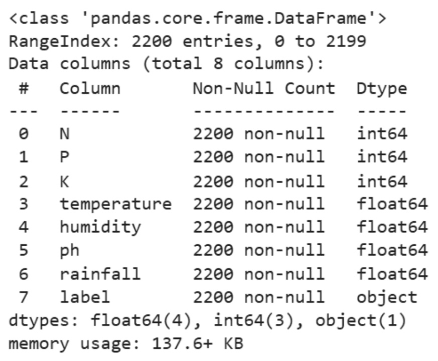
The dataset behind it is modest: about 2,200 rows. But it covers important details like soil nutrients (nitrogen, phosphorus, potassium) and pH levels, plus basic climate information like temperature, humidity, and rainfall. Here is a sample of the data:

Instead of reaching for deep learning or other heavy methods, the analysis stays intentionally simple.
We start with some descriptive statistics:
|
df.select_dtypes(include=[‘int64’, ‘float64’]).describe() |

Then, we proceed to some visual exploration:
|
1 2 3 4 5 6 7 8 9 10 11 12 13 14 15 16 17 18 19 20 |
# Setting the aesthetic style of the plots sns.set_theme(style=“whitegrid”)
# Creating visualizations for Temperature, Humidity, and Rainfall fig, axes = plt.subplots(1, 3, figsize=(14, 5))
# Temperature Distribution sns.histplot(df[‘temperature’], kde=True, color=“skyblue”, ax=axes[0]) axes[0].set_title(‘Temperature Distribution’)
# Humidity Distribution sns.histplot(df[‘humidity’], kde=True, color=“olive”, ax=axes[1]) axes[1].set_title(‘Humidity Distribution’)
# Rainfall Distribution sns.histplot(df[‘rainfall’], kde=True, color=“gold”, ax=axes[2]) axes[2].set_title(‘Rainfall Distribution’)
plt.tight_layout() plt.show() |

Finally, we run a few ANOVA tests to understand how environmental factors differ across crop types:
ANOVA Analysis for Humidity
|
# Define crop_types based on your DataFrame ‘df’ crop_types = df[‘label’].unique()
# Preparing a list of humidity values for each crop type humidity_lists = [df[df[‘label’] == crop][‘humidity’] for crop in crop_types]
# Performing the ANOVA test for humidity anova_result_humidity = f_oneway(*humidity_lists)
anova_result_humidity |

ANOVA Analysis for Rainfall
|
# Define crop_types based on your DataFrame ‘df’ if not already defined crop_types_rainfall = df[‘label’].unique()
# Preparing a list of rainfall values for each crop type rainfall_lists = [df[df[‘label’] == crop][‘rainfall’] for crop in crop_types_rainfall]
# Performing the ANOVA test for rainfall anova_result_rainfall = f_oneway(*rainfall_lists)
anova_result_rainfall |

ANOVA Analysis for Temperature
|
# Ensure crop_types is defined from your DataFrame ‘df’ crop_types_temp = df[‘label’].unique()
# Preparing a list of temperature values for each crop type temperature_lists = [df[df[‘label’] == crop][‘temperature’] for crop in crop_types_temp]
# Performing the ANOVA test for temperature anova_result_temperature = f_oneway(*temperature_lists)
anova_result_temperature |

This small-scale, low-resource project mirrors real-life challenges in rural farming. We all know that weather patterns do not follow rules, and climate data can be patchy or inconsistent. So, instead of throwing a complex model at the problem and hoping it figures things out, we dug into the data manually.
Perhaps the most valuable aspect of this approach is its interpretability. Farmers are not looking for opaque predictions; they want guidance they can act on. Statements like “this crop performs better under high humidity” or “that crop tends to prefer drier conditions” translate statistical findings into practical decisions.
This entire workflow was super lightweight. No fancy hardware, no expensive software, just trusty tools like pandas, Seaborn, and some basic statistical tests. Everything ran smoothly on a regular laptop.
The core analytical step used ANOVA to check whether environmental conditions such as humidity or rainfall vary significantly between crop types.
In many ways, this captures the spirit of machine learning in low-resource environments. The techniques remain grounded, computationally gentle, and easy to explain, yet they still offer insights that can help people make more informed decisions, even without advanced infrastructure.
For Aspiring Data Scientists in Low-Resource Settings
You might not have a GPU. You might be using free-tier tools. And your data might look like a puzzle with missing pieces.
But here’s the thing: you’re learning skills that many overlook:
- Real-world data cleaning
- Feature engineering with instinct
- Building trust through explainable models
- Working smart, not flashy
Prioritize this:
- Clean, consistent data
- Classic models that work
- Thoughtful features
- Simple transfer learning tricks
- Clear notes and reproducibility
In the end, this is the kind of work that makes a great data scientist.
Conclusion
Image by Author
Working in low-resource machine learning environments is possible. It asks you to be creative and passionate about your mission. It comes down to finding the signal in the noise and solving real problems that make life easier for real people.
In this article, we explored how lightweight models, smart features, honest handling of missing data, and clever reuse of existing knowledge can help you get ahead when working in this type of situation.
What are your thoughts? Have you ever built a solution in a low-resource setup?