A Gentle Introduction to Batch Normalization

A Gentle Introduction to Batch Normalization
Image by Editor | ChatGPT

Introduction

Deep neural networks have drastically evolved over the years, overcoming common challenges that arise when training these complex models. This evolution has enabled them to solve increasingly difficult problems effectively.

One of the mechanisms that has proven especially influential in the advancement of neural network-based models is batch normalization. This article provides a gentle introduction to this strategy, which has become a standard in many modern architectures, helping to improve model performance by stabilizing training, speeding up convergence, and more.

How and Why Batch Normalization Was Born?

Batch normalization is roughly 10 years old. It was originally proposed by Ioffe and Szegedy in their paper Batch Normalization: Accelerating Deep Network Training by Reducing Internal Covariate Shift.

The motivation for its creation stemmed from several challenges, including slow training processes and saturation issues like exploding and vanishing gradients. One particular challenge highlighted in the original paper is internal covariate shift: in simple terms, this issue is related to how the distribution of inputs to each layer of neurons keeps changing during training iterations, largely because the learnable parameters (connection weights) in the previous layers are naturally being updated during the entire training process. These distribution shifts might trigger a sort of “chicken and egg” problem, as they force the network to keep readjusting itself, sometimes leading to unduly slow and unstable training.

How Does it Work?

In response to the aforementioned issue, batch normalization was proposed as a method that normalizes the inputs to layers in a neural network, helping stabilize the training process as it progresses.

In practice, batch normalization entails introducing an additional normalization step before the assigned activation function is applied to weighted inputs in such layers, as shown in the diagram below.

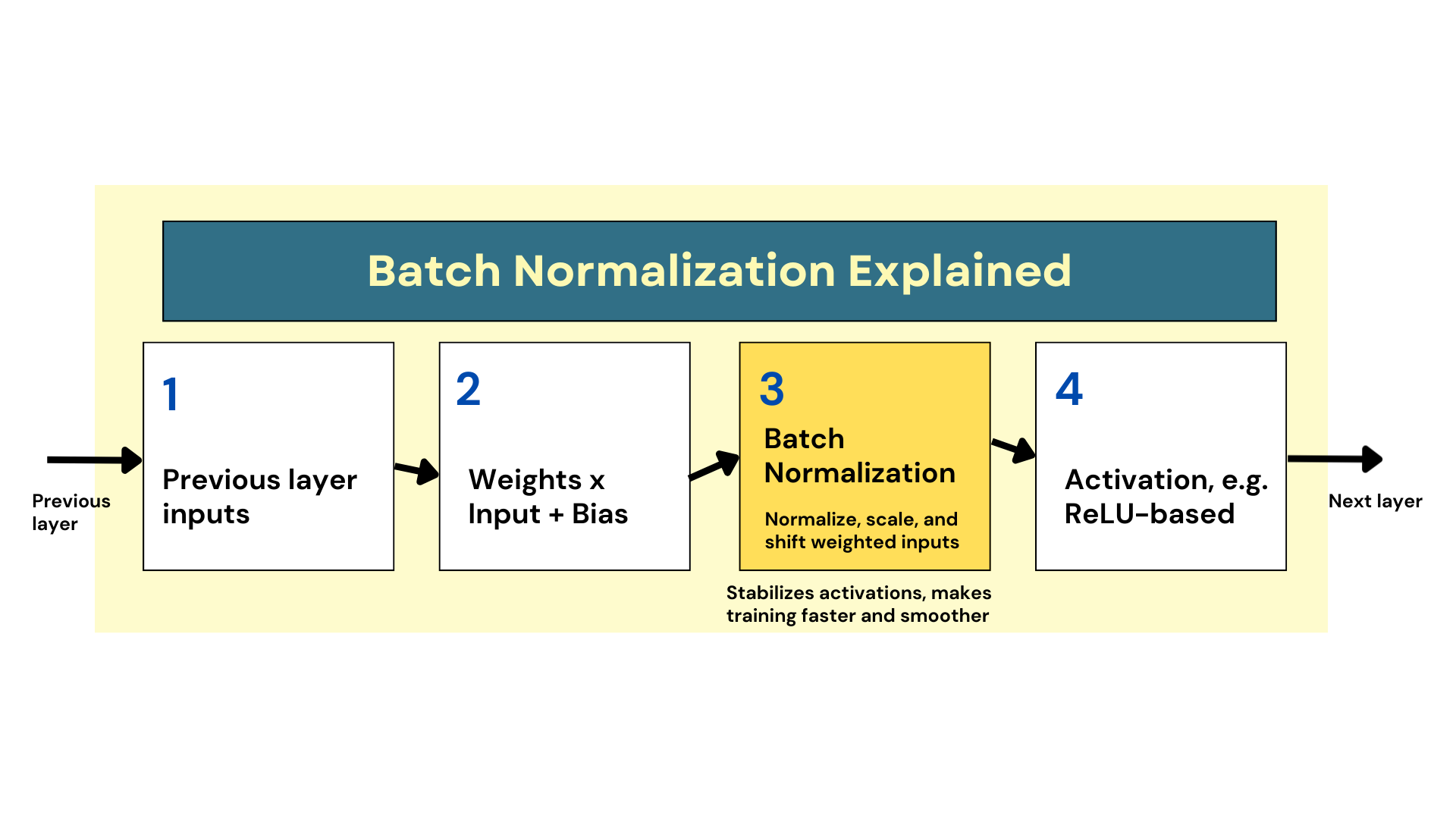
How Batch Normalization Works
Image by Author

In its simplest form, the mechanism consists of zero-centering, scaling, and shifting the inputs so that values stay within a more consistent range. This simple idea helps the model learn an optimal scale and mean for inputs at the layer level. Consequently, gradients that flow backward to update weights during backpropagation do so more smoothly, reducing side effects like sensitivity to the weight initialization method, e.g., He initialization. And most importantly, this mechanism has proven to facilitate faster and more reliable training.

At this point, two typical questions may arise:

1. Why the “batch” in batch normalization?: If you are fairly familiar with the basics of training neural networks, you may know that the training set is partitioned into mini-batches — typically containing 32 or 64 instances each — to speed up and scale the optimization process underlying training. Thus, the technique is so named because the mean and variance used for normalization of weighted inputs are not calculated over the entire training set, but rather at the batch level.
2. Can it be applied to all layers in a neural network?: Batch normalization is normally applied to the hidden layers, which is where activations can destabilize during training. Since raw inputs are usually normalized beforehand, it is rare to apply batch normalization in the input layer. Likewise, applying it to the output layer is counterproductive, as it may break the assumptions made for the expected range for the output’s values, especially for instance in regression neural networks for predicting aspects like flight prices, rainfall amounts, and so on.

A major positive impact of batch normalization is a strong reduction in the vanishing gradient problem. It also provides more robustness, reduces sensitivity to the chosen weight initialization method, and introduces a regularization effect. This regularization helps combat overfitting, sometimes eliminating the need for other specific strategies like dropout.

How to Implement it in Keras

Keras is a popular Python API on top of TensorFlow used to build neural network models, where designing the architecture is an essential step before training. This example shows how simple it is to implement batch normalization in a simple neural network to be trained with Keras:

Introducing this strategy is as simple as adding BatchNormalization() between the layer definition and its associated activation function. The input layer in this example is not explicitly defined, with the first dense layer acting as the first hidden layer that receives pre-normalized raw inputs.

Importantly, note that incorporating batch normalization forces us to define each subcomponent in the layer separately, no longer being able to specify the activation function as an argument inside the layer definition, e.g., Dense(32, activation='relu'). Still, conceptually speaking, the three lines of code can still be interpreted as one neural network layer instead of three, even though Keras and TensorFlow internally manage them as separate sublayers.

Wrapping Up

This article provided a gentle and approachable introduction to batch normalization: a simple yet very effective mechanism that often helps alleviate some common problems found when training neural network models. Simple terms (or at least I tried to!), no math here and there, and for those a bit more tech-savvy, a final (also gentle) example of how to implement it in Python.