

In this article, you will learn how to choose an appropriate time series forecasting model using a clear, four-quadrant decision matrix grounded in data complexity and input dimensionality.
Topics we will cover include:
- The difference between univariate and multivariate time series and why it matters.
- Which classical and modern models fit best for low vs. high complexity data.
- Trade-offs among interpretability, scalability, and accuracy across model families.
Let’s not waste any more time.
A Decision Matrix for Time Series Forecasting Models
Image by Editor
Introduction
Time series data have the added complexity of temporal dependencies, seasonality, and possible non-stationarity.
Arguably, the most frequent predictive problem to address with time series data is forecasting i.e. predicting future values of a variable like temperature or stock price based on historical observations up to the present. With so many different models for time series forecasting, practitioners might sometimes find it difficult to choose the most suitable approach.
This article is designed to help, through the use of a decision matrix accompanied by explanations on when and why to employee different models depending on data characteristics and problem type.
The Decision Matrix
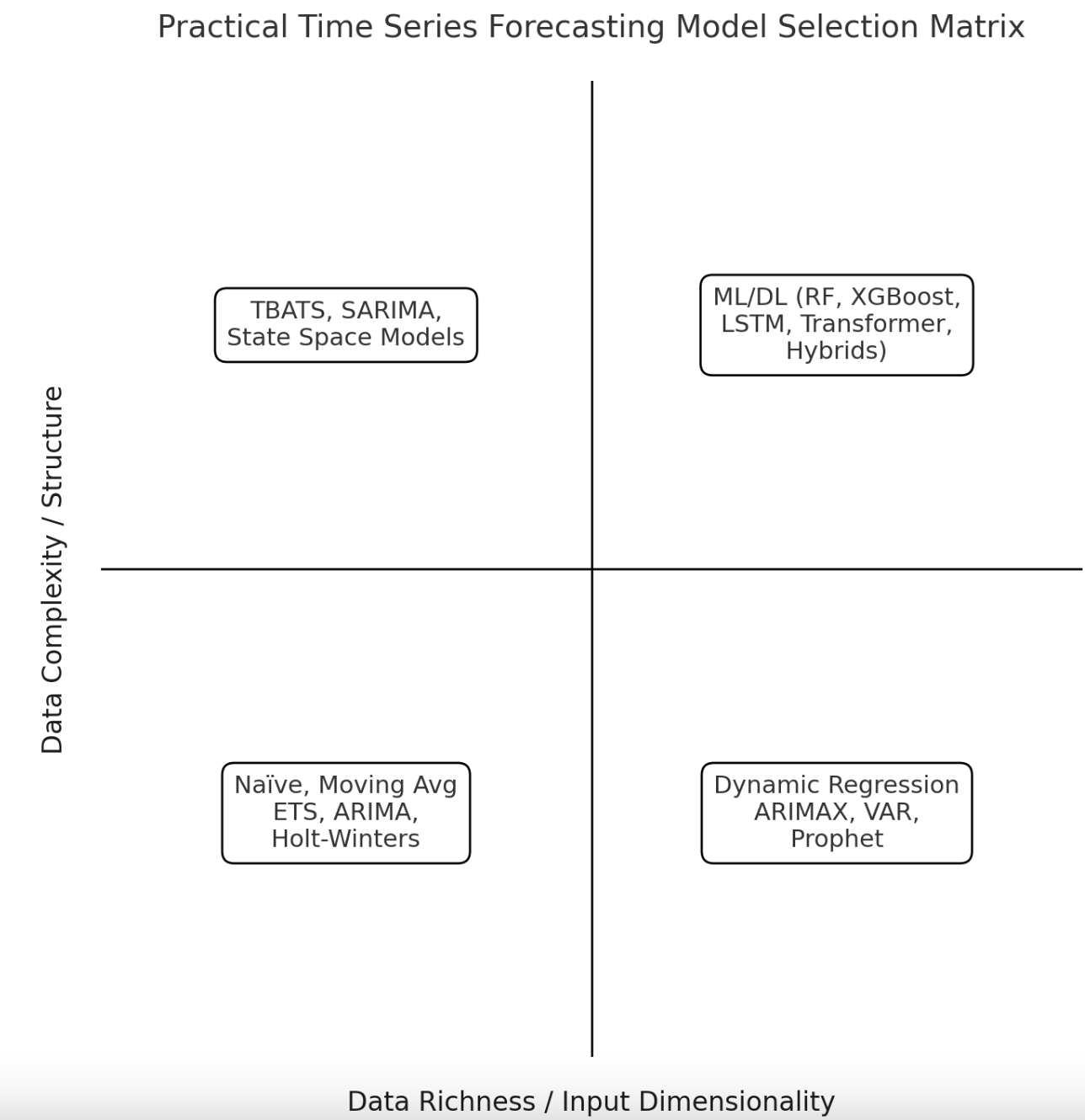
First up, we introduce the visual matrix that categorizes a set of commonly used time series forecasting models depending on two major criteria or dimensions.
A Decision Matrix for Time Series Forecasting Models
Image by Author
Data complexity and structure refers to the overall complexity of the time series dataset being used, in terms of aspects like the presence or absence of stationarity patterns, seasonality, limited vs. significant noise in the data, nonlinearities, and so on.
Input dimensionality refers to the fact that, based on input data dimensionality, the time series can be univariate or multivariate i.e. without or with exogenous input attributes, respectively. For instance, a dataset describing daily rides in a public transport system would be an example of a univariate time series, whereas daily or hourly weather recordings including wind speed, temperature, and humidity are an example of a multivariate time series.
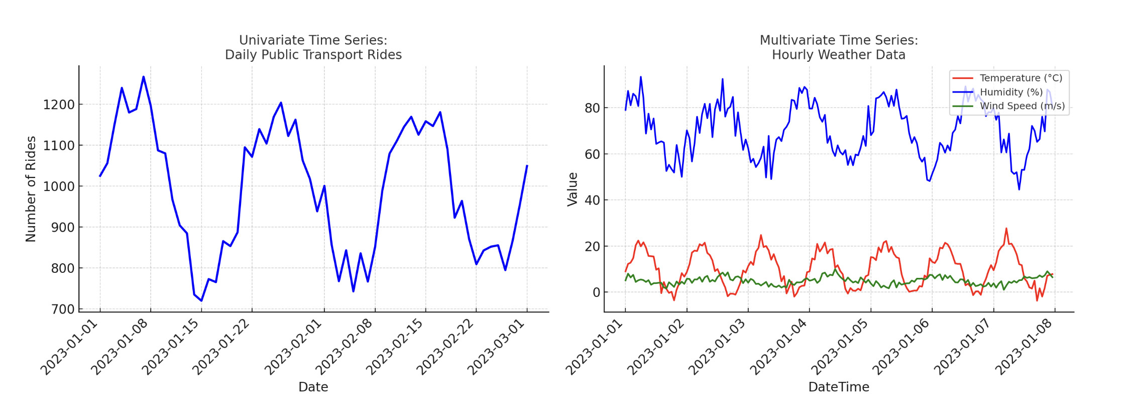
Univariate vs Multivariate Time Series
Image by Author
These two classification criteria lead us to a taxonomy of time series forecasting models aligned with the matrix displayed above.
Let’s now look into each of the four quadrants in more detail.
1. Low-Complexity, Univariate Time Series (Bottom Left)
This quadrant encompasses forecasting problems where the historical time series has low complexity — for instance, because it is rather short, it has stable demand (fairly constant over time), or it exhibits simple trends, patterns, or seasonal structure. Normally, these kinds of time series also display approximate stationarity.
Suitable and simple models that are normally enough for these problems include Naïve (for extremely simplistic time series data), or slightly more elaborate algorithms or techniques like moving averages and their variants (simple moving average, weighted moving average), the classic among the classics autoregressive integrated moving average (ARIMA), and Holt–Winters. These are all robust models for simple time series datasets, while keeping interpretability and efficiency in forecasts. Meanwhile, due to their simplicity compared to other advanced approaches, their adaptability to issues such as structural breaks or external factors is very limited.
2. Low-Complexity, Multivariate Time Series (Bottom Right)
When the time series still has simple patterns but is multivariate — or it is influenced by multiple external factors or regression predictors — it is better to resort to intermediate-complexity models like Dynamic Regression, ARIMA with exogenous variables (ARIMAX), vector autoregression (VAR), or Prophet. These forecasting models can directly incorporate known drivers — such as promotions or pricing effects in customer historical behavior data — into the forecasting, thereby acting as a hybrid between purely time-based forecasting and regression models.
These approaches are generally easy to interpret and implement, generating reliable predictions when the underlying dynamics of the dataset remain relatively straightforward. On the other hand, despite being able to incorporate external variables, they still assume relatively simple patterns and relationships and may struggle with nonlinearities or hard-to-understand interactions among variables.
3. High-Complexity, Univariate Time Series (Top Left)
Univariate time series exhibiting complex patterns — like irregular trends or multiple seasonal cycles — require using specialized models like TBATS (Trigonometric, Box–Cox transformation, ARMA errors, Trend, and Seasonal components), seasonal ARIMA (SARIMA), or state-space methods such as Kalman filter–based approaches. Aspects like non-stationarity i.e. evolving statistical properties of the data over time, and complex seasonal behaviors can be captured by these models, which makes them suitable for forecasting in scenarios with long-term or irregular series with somewhat “unpredictable” dynamics.
Although they outperform other models in coping with internal complexities, these methods are more computationally intensive, and in practice, they often require careful fine-tuning to be precise and generalizable.
4. High-Complexity, Multivariate Time Series (Top Right)
Last of the four scenarios, we have contexts with large time series that contain multiple time and/or external variables and present complex or nonlinear dependencies. These challenging scenarios require advanced techniques from the machine learning and deep learning landscape — for example, ensemble methods like Random Forests and XGBoost, recurrent neural networks such as long short-term memory (LSTM) networks, or even deep learning architectures like transformers. Nonetheless, using hybrid approaches is often a wise choice in these contexts.
These data-intensive models are superior at capturing complex interactions among variables and are scalable to very large datasets. But on the negative side of things, their requirements are more demanding and they have lower interpretability, along with some risk of overfitting if not enough high-quality data is provided to train them.
Wrapping Up
This article took a tour of time series forecasting models and methods from the perspective of practical choice. Based on a four-quadrant decision matrix, we outlined the preferred methods to use in four different types of forecasting scenarios, highlighting when to use each group of models and outlining the pros and cons of each.