Linear Layers and Activation Functions in Transformer Models

Attention operations are the signature of transformer models, but they are not the only building blocks. Linear layers and activation functions are equally essential. In this post, you will learn about:

• Why linear layers and activation functions enable non-linear transformations
• The typical design of feed-forward networks in transformer models
• Common activation functions and their characteristics

Let’s get started.

Overview

This post is divided into three parts; they are:

• Why Linear Layers and Activations are Needed in Transformers
• Typical Design of the Feed-Forward Network
• Variations of the Activation Functions

Why Linear Layers and Activations are Needed in Transformers

The attention layer is the core function of a transformer model. It aligns different elements in a sequence and transforms the input sequence into an output sequence. The attention layer performs an affine transformation of the input, meaning the output is a weighted sum of the input at each sequence element.

Neural networks derive their power not from linear layers alone, but from activation functions that introduce non-linearity. In transformer models, you need non-linearity after the attention layer to learn complex patterns. This is achieved by adding a feed-forward network (FFN) or multi-layer perception network (MLP) after each attention layer. A typical transformer block looks like this:

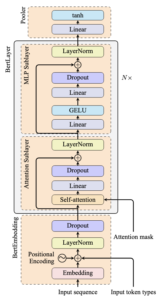
Architecture of the BERT model

The gray box in the figure above repeats multiple times in a transformer model. In each block (excluding normalization layers), the input first passes through an attention layer, then through a feed-forward network (implemented as nn.Linear in PyTorch). An activation function within the feed-forward network adds non-linearity to the transformation.

The feed-forward network allows the model to learn more complex patterns. Typically, it contains multiple linear layers: the first expands the dimension to explore different representations, while the last contracts it back to the original dimension. Activations are usually applied to the output of the first linear layer.

Due to this design, we typically call the first half of the block the “attention sub-layer” and the second half the “MLP sub-layer.”

Typical Design of the Feed-Forward Network

In the BERT model, the MLP sublayer is implemented as follows:

The MLP sublayer contains two linear modules. When an input sequence enters the MLP sublayer, the first linear module expands the dimension, then applies the GELU activation function. The result passes through the second linear module to contract the dimension back to the original size.

The intermediate dimension is typically 4 times the original dimension: a common design pattern in transformer models.

Variations of the Activation Functions

Activation functions introduce non-linearity into neural networks, enabling them to learn complex patterns. While traditional neural networks commonly use hyperbolic tangent (tanh), sigmoid, and rectified linear unit (ReLU), transformer models typically employ GELU and SwiGLU activations.

Below are the mathematical definitions of some common activation functions:

$$
\begin{aligned}
\text{Sigmoid}(x) &= \frac{1}{1 + e^{-x}} \\
\tanh(x) &= \frac{e^x – e^{-x}}{e^x + e^{-x}} = 2\text{Sigmoid}(2x) – 1 \\
\text{ReLU}(x) &= \max(0, x) \\
\text{GELU}(x) &= x \cdot \Phi(x) \approx \frac{x}{2}\Big(1 + \tanh\big(\sqrt{\frac{2}{\pi}}(x + 0.044715x^3)\big)\Big) \\
\text{Swish}_\beta(x) &= x \cdot \text{Sigmoid}(\beta x) = \frac{x}{1 + e^{-\beta x}} \\
\text{SiLU}(x) &= \frac{x}{1 + e^{-x}} = \text{Swish}_1(x) \\
\text{SwiGLU}(x) &= \text{SiLU}(xW + b) \cdot (xV + c)
\end{aligned}
$$

ReLU (rectified linear unit) is popular in modern deep learning because it avoids the vanishing gradient problem and is computationally simple.

GELU (Gaussian Error Linear Unit) is more computationally expensive due to its use of the cumulative distribution function of the standard normal distribution $\Phi(x)$. An approximation formula exists, as shown above. GELU is not monotonic, as you can see in the figure below.

Monotonic activation functions are generally preferred because they ensure consistent gradient direction, potentially leading to faster convergence. However, monotonicity is not strictly required—you may just need longer training times. You trade off model complexity with training duration.

Swish is another non-monotonic activation function with a parameter $\beta$ that controls the slope at $x=0$. When $\beta=1$, it’s called SiLU (Sigmoid Linear Unit).

SwiGLU (Swish-Gated Linear Unit) is a recent activation function common in modern transformer models. It’s the product of a Swish function and a linear function, with parameters learned during training. Its popularity stems from its complexity: expanding the formula reveals a quadratic term in the numerator, helping models learn complex patterns without additional layers.

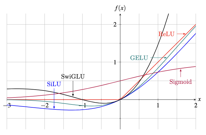
Plot of some common activation functions

The figure above shows plots of these activation functions. The SwiGLU function shown is $f(x) = \text{SiLU}(x) \cdot (x+1)$.

Switching activation functions in the Python code is straightforward. PyTorch provides built-in nn.Sigmoid, nn.ReLU, nn.Tanh, and nn.SiLU. However, SwiGLU requires special implementation. Below is the PyTorch code used in the Llama model:

This implementation uses two linear layers to process the input hidden_states. One output passes through the SiLU function, then multiplies with the other output before processing through a final linear layer. The linear layers are named “up” or “down” for dimension expansion/contraction, while the layer connected to SiLU is called “gate” for its gating mechanism. Gating is a design of the neural network that means the elementwise multiplication of the output of one linear layer by a weight, which here is produced by the Swish activation function.

The Llama model architecture appears as follows, showing the MLP module’s dual-branch structure:

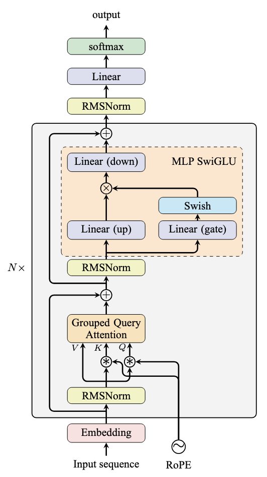
Architecture of a Llama model

Further Readings

Below are some resources that you may find useful:

Summary

In this post, you learned about linear layers and activation functions in transformer models. Specifically, you learned about:

• Why linear layers and activation functions are necessary for non-linear transformations
• The characteristics and implementations of ReLU, GELU, and SwiGLU activation functions
• How to build complete feed-forward networks as used in transformer models