

In this article, you will learn practical, safe ways to use data augmentation to reduce overfitting and improve generalization across images, text, audio, and tabular datasets.
Topics we will cover include:
- How augmentation works and when it helps.
- Online vs. offline augmentation strategies.
- Hands-on examples for images (TensorFlow/Keras), text (NLTK), audio (librosa), and tabular data (NumPy/Pandas), plus the critical pitfalls of data leakage.
Alright, let’s get to it.
The Complete Guide to Data Augmentation for Machine Learning
Image by Author
Suppose you’ve built your machine learning model, run the experiments, and stared at the results wondering what went wrong. Training accuracy looks great, maybe even impressive, but when you check validation accuracy… not so much. You can solve this issue by getting more data. But that is slow, expensive, and sometimes just impossible.
It’s not about inventing fake data. It’s about creating new training examples by subtly modifying the data you already have without changing its meaning or label. You’re showing your model the same concept in multiple forms. You are teaching what’s important and what can be ignored. Augmentation helps your model generalize instead of simply memorizing the training set. In this article, you’ll learn how data augmentation works in practice and when to use it. Specifically, we’ll cover:
- What data augmentation is and why it helps reduce overfitting
- The difference between offline and online data augmentation
- How to apply augmentation to image data with TensorFlow
- Simple and safe augmentation techniques for text data
- Common augmentation methods for audio and tabular datasets
- Why data leakage during augmentation can silently break your model
Offline vs Online Data Augmentation
Augmentation can happen before training or during training. Offline augmentation expands the dataset once and saves it. Online augmentation generates new variations every epoch. Deep learning pipelines usually prefer online augmentation because it exposes the model to effectively unbounded variation without increasing storage.
Data Augmentation for Image Data
Image data augmentation is the most intuitive place to start. A dog is still a dog if it’s slightly rotated, zoomed, or viewed under different lighting conditions. Your model needs to see these variations during training. Some common image augmentation techniques are:
- Rotation
- Flipping
- Resizing
- Cropping
- Zooming
- Shifting
- Shearing
- Brightness and contrast changes
These transformations do not change the label—only the appearance. Let’s demonstrate with a simple example using TensorFlow and Keras:
1. Importing Libraries
|
import tensorflow as tf from tensorflow.keras.datasets import mnist from tensorflow.keras.layers import Dense, Flatten, Conv2D, MaxPooling2D, Dropout from tensorflow.keras.utils import to_categorical from tensorflow.keras.preprocessing.image import ImageDataGenerator from tensorflow.keras.models import Sequential |
2. Loading MNIST dataset
|
(X_train, y_train), (X_test, y_test) = mnist.load_data()
# Normalize pixel values X_train = X_train / 255.0 X_test = X_test / 255.0
# Reshape to (samples, height, width, channels) X_train = X_train.reshape(–1, 28, 28, 1) X_test = X_test.reshape(–1, 28, 28, 1)
# One-hot encode labels y_train = to_categorical(y_train, 10) y_test = to_categorical(y_test, 10) |
Output:
|
Downloading data from https://storage.googleapis.com/tensorflow/tf-keras-datasets/mnist.npz |
3. Defining ImageDataGenerator for augmentation
|
datagen = ImageDataGenerator( rotation_range=15, # rotate images by ±15 degrees width_shift_range=0.1, # 10% horizontal shift height_shift_range=0.1, # 10% vertical shift zoom_range=0.1, # zoom in/out by 10% shear_range=0.1, # apply shear transformation horizontal_flip=False, # not needed for digits fill_mode=‘nearest’ # fill missing pixels after transformations ) |
4. Building a Simple CNN Model
|
model = Sequential([ Conv2D(32, (3, 3), activation=‘relu’, input_shape=(28, 28, 1)), MaxPooling2D((2, 2)), Conv2D(64, (3, 3), activation=‘relu’), MaxPooling2D((2, 2)), Flatten(), Dropout(0.3), Dense(64, activation=‘relu’), Dense(10, activation=‘softmax’) ])
model.compile(optimizer=‘adam’, loss=‘categorical_crossentropy’, metrics=[‘accuracy’]) |
5. Training the model
|
batch_size = 64 epochs = 5
history = model.fit( datagen.flow(X_train, y_train, batch_size=batch_size, shuffle=True), steps_per_epoch=len(X_train)//batch_size, epochs=epochs, validation_data=(X_test, y_test) ) |
Output:
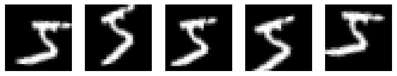
6. Visualizing Augmented Images
|
import matplotlib.pyplot as plt
# Visualize five augmented variants of the first training sample plt.figure(figsize=(10, 2)) for i, batch in enumerate(datagen.flow(X_train[:1], batch_size=1)): plt.subplot(1, 5, i + 1) plt.imshow(batch[0].reshape(28, 28), cmap=‘gray’) plt.axis(‘off’) if i == 4: break plt.show() |
Output:
Data Augmentation for Textual Data
Text is more delicate. You can’t randomly replace words without thinking about meaning. But small, controlled changes can help your model generalize. A simple example using synonym replacement (with NLTK):
|
1 2 3 4 5 6 7 8 9 10 11 12 13 14 15 16 17 18 19 20 |
import nltk from nltk.corpus import wordnet import random
nltk.download(“wordnet”) nltk.download(“omw-1.4”)
def synonym_replacement(sentence): words = sentence.split() if not words: return sentence idx = random.randint(0, len(words) – 1) synsets = wordnet.synsets(words[idx]) if synsets and synsets[0].lemmas(): replacement = synsets[0].lemmas()[0].name().replace(“_”, ” “) words[idx] = replacement return ” “.join(words)
text = “The movie was really good” print(synonym_replacement(text)) |
Output:
|
[nltk_data] Downloading package wordnet to /root/nltk_data... The movie was truly good |
Same meaning. New training example. In practice, libraries like nlpaug or back-translation APIs are often used for more reliable results.
Data Augmentation for Audio Data
Audio data also benefits heavily from augmentation. Some common audio augmentation techniques are:
- Adding background noise
- Time stretching
- Pitch shifting
- Volume scaling
One of the simplest and most commonly used audio augmentations is adding background noise and time stretching. These help speech and sound models perform better in noisy, real-world environments. Let’s understand with a simple example (using librosa):
|
1 2 3 4 5 6 7 8 9 10 11 12 13 14 15 16 17 18 |
import librosa import numpy as np
# Load built-in trumpet audio from librosa audio_path = librosa.ex(“trumpet”) audio, sr = librosa.load(audio_path, sr=None)
# Add background noise noise = np.random.randn(len(audio)) audio_noisy = audio + 0.005 * noise
# Time stretching audio_stretched = librosa.effects.time_stretch(audio, rate=1.1)
print(“Sample rate:”, sr) print(“Original length:”, len(audio)) print(“Noisy length:”, len(audio_noisy)) print(“Stretched length:”, len(audio_stretched)) |
Output:
|
Downloading file ‘sorohanro_-_solo-trumpet-06.ogg’ from ‘https://librosa.org/data/audio/sorohanro_-_solo-trumpet-06.ogg’ to ‘/root/.cache/librosa’. Sample rate: 22050 Original length: 117601 Noisy length: 117601 Stretched length: 106910 |
You should observe that the audio is loaded at 22,050 Hz. Now, adding noise does not change its length, so the noisy audio is the same size as the original. Time stretching speeds up the audio while preserving content.
Data Augmentation for Tabular Data
Tabular data is the most sensitive data type to augment. Unlike images or audio, you cannot arbitrarily modify values without breaking the data’s logical structure. However, some common augmentation techniques exist:
- Noise Injection: Add small, random noise to numerical features while preserving the overall distribution.
- SMOTE: Generates synthetic samples for minority classes in classification problems.
- Mixing: Combine rows or columns in a way that maintains label consistency.
- Domain-Specific Transformations: Apply logic-based changes depending on the dataset (e.g., converting currencies, rounding, or normalizing).
- Feature Perturbation: Slightly alter input features (e.g., age ± 1 year, income ± 2%).
Now, let’s understand with a simple example using noise injection for numerical features (via NumPy and Pandas):
|
1 2 3 4 5 6 7 8 9 10 11 12 13 14 15 16 17 18 19 20 21 |
import numpy as np import pandas as pd
# Sample tabular dataset data = { “age”: [25, 30, 35, 40], “income”: [40000, 50000, 60000, 70000], “credit_score”: [650, 700, 750, 800] }
df = pd.DataFrame(data)
# Add small Gaussian noise to numerical columns augmented_df = df.copy() noise_factor = 0.02 # 2% noise
for col in augmented_df.columns: noise = np.random.normal(0, noise_factor, size=len(df)) augmented_df[col] = augmented_df[col] * (1 + noise)
print(augmented_df) |
Output:
|
age income credit_score 0 24.399643 41773.983250 651.212014 1 30.343270 50962.007818 696.959347 2 34.363792 58868.638800 757.656837 3 39.147648 69852.508717 780.459666 |
You can see that this slightly modifies the numerical values but preserves the overall data distribution. It also helps the model generalize instead of memorizing exact values.
The Hidden Danger of Data Leakage
This part is non-negotiable. Data augmentation must be applied only to the training set. You should never augment validation or test data. If augmented data leaks into the evaluation, your metrics become misleading. Your model will look great on paper and fail in production. Clean separation is not a best practice; it’s a requirement.
Conclusion
Data augmentation helps when your data is limited, overfitting is present, and real-world variation exists. It does not fix incorrect labels, biased data, or poorly defined features. That’s why understanding your data always comes before applying transformations. It isn’t just a trick for competitions or deep learning demos. It’s a mindset shift. You don’t need to chase more data, but you have to start asking how your existing data might naturally change. Your models stop overfitting, start generalizing, and finally behave the way you expected them to in the first place.