

10 Python One-Liners for Generating Time Series Features
Introduction
Time series data normally requires an in-depth understanding in order to build effective and insightful forecasting models. Two key properties are critical in time series forecasting: representation and granularity.
- Representation entails using meaningful approaches to transform raw temporal data — e.g. daily or hourly measurements — into informative patterns
- Granularity is about analyzing how precisely such patterns capture variations across time.
As two sides of the same coin, their difference is subtle, but one thing is certain: both are achieved through feature engineering.
This article presents 10 simple Python one-liners for generating time series features based on different characteristics and properties underlying raw time series data. These one-liners can be used in isolation or in combination to help you create more informative datasets that reveal much about your data’s temporal behavior — how it evolves, how it fluctuates, and which trends it exhibits over time.
Note that our examples make use of Pandas and NumPy.
1. Lag Feature (Autoregressive Representation)
The idea behind using autoregressive representation or lag features is simpler than it sounds: it consists of adding the previous observation as a new predictor feature in the current observation. In essence, this is arguably the simplest method to represent temporal dependency, e.g. between the current time instant and previous ones.
As the first one-liner example code in this list of 10, let’s look at this one more closely.
This example one-liner assumes you have stored a raw time series dataset in a DataFrame called df, one of whose existing attributes is named 'value'. Note that the argument in the shift() function can be adjusted to fetch the value registered n time instants or observations before the current one:
|
df[‘lag_1’] = df[‘value’].shift(1) |
For daily time series data, if you wanted to capture previous values for a given day of the week, e.g. Monday, it would make sense to use shift(7).
2. Rolling Mean (Short-Term Smoothing)
To capture local trends or smoother short-term fluctuations in the data, it is usually handy to use rolling means across the n past observations leading to the current one: this is a simple but very useful way to smooth sometimes chaotic raw time series values over a given feature.
This example creates a new feature containing, for each observation, the rolling mean of the three previous values of this feature in recent observations:
|
df[‘rolling_mean_3’] = df[‘value’].rolling(3).mean() |
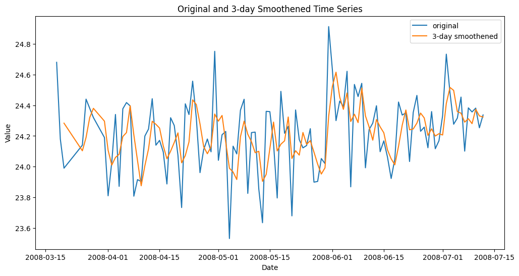
Smoothed time series feature with rolling mean
3. Rolling Standard Deviation (Local Volatility)
Similar to rolling means, there is also the possibility of creating new features based on rolling standard deviation, which is effective for modeling how volatile consecutive observations are.
This example introduces a feature to model the variability of the latest values over a moving window of a week, assuming daily observations.
|
df[‘rolling_std_7’] = df[‘value’].rolling(7).std() |
4. Expanding Mean (Cumulative Memory)
The expanding mean calculates the mean of all data points up to (and including) the current observation in the temporal sequence. Hence, it is like a rolling mean with a constantly increasing window size. It is useful to analyze how the mean of values in a time series attribute evolves over time, thereby capturing upward or downward trends more reliably in the long term.
|
df[‘expanding_mean’] = df[‘value’].expanding().mean() |
5. Differencing (Trend Removal)
This technique is used to remove long-term trends, highlighting change rates — important in non-stationary time series to stabilize them. It calculates the difference between consecutive observations (current and previous) of a target attribute:
|
df[‘diff_1’] = df[‘value’].diff() |
6. Time-Based Features (Temporal Component Extraction)
Simple but very useful in real-world applications, this one-liner can be used to decompose and extract relevant information from the full date-time feature or index your time series revolves around:
|
df[‘month’], df[‘dayofweek’] = df[‘Date’].dt.month, df[‘Date’].dt.dayofweek |
Important: Be careful and check whether in your time series the date-time information is contained in a regular attribute or as the index of the data structure. If it were the index, you may need to use this instead:
|
df[‘hour’], df[‘dayofweek’] = df.index.hour, df.index.dayofweek |
7. Rolling Correlation (Temporal Relationship)
This approach takes a step beyond rolling statistics over a time window to measure how recent values correlate with their lagged counterparts, thereby helping discover evolving autocorrelation. This is useful, for example, in detecting regime shifts, i.e. abrupt and persistent behavioral changes in the data over time, which take place when rolling correlations start to weaken or reverse at some point.
|
df[‘rolling_corr’] = df[‘value’].rolling(30).corr(df[‘value’].shift(1)) |
8. Fourier Features (Seasonality)
Sinusoidal Fourier transformations can be used in raw time series attributes to capture cyclic or seasonal patterns. For example, applying the sine (or cosine) function transforms cyclical day-of-year information underlying date-time features into continuous features useful for learning and modeling yearly patterns.
|
df[‘fourier_sin’] = np.sin(2 * np.pi * df[‘Date’].dt.dayofyear / 365) df[‘fourier_cos’] = np.cos(2 * np.pi * df[‘Date’].dt.dayofyear / 365) |
Allow me to use a two-liner, instead of a one-liner in this example, for a reason: both sine and cosine together are better at capturing the big picture of possible cyclic seasonality patterns.
9. Exponentially Weighted Mean (Adaptive Smoothing)
The exponentially weighted mean — or EWM for short — is applied to obtain exponentially decaying weights that give higher importance to recent data observations while still retaining long-term memory. It is a more adaptive and somewhat “smarter” approach that prioritizes recent observations over the distant past.
|
df[‘ewm_mean’] = df[‘value’].ewm(span=5).mean() |
10. Rolling Entropy (Information Complexity)
A bit more math for the last one! The rolling entropy of a given feature over a time window calculates how random or spread out the values over that time window are, thereby revealing the quantity and complexity of information in it. Lower values of the resulting rolling entropy indicate a sense of order and predictability, whereas the higher these values are, the more the “chaos and uncertainty.”
|
df[‘rolling_entropy’] = df[‘value’].rolling(10).apply(lambda x: –np.sum((p:=np.histogram(x, bins=5)[0]/len(x))*np.log(p+1e–9))) |
Wrapping Up
In this article, we have examined and illustrated 10 strategies — spanning a single line of code each — to extract a variety of patterns and information from raw time series data, from simpler trends to more sophisticated ones like seasonality and information complexity.