The Beginner’s Guide to Clustering with Python
Image by Author | Ideogram
Clustering is a widely applied method in many domains like customer and image segmentation, image recognition, bioinformatics, and anomaly detection, all to group data into clusters in terms of similarity. Clustering methods have a double-sided nature: as a machine learning technique aimed at discovering knowledge underneath unlabeled data (unsupervised learning), and as a descriptive data analysis tool for uncovering hidden patterns in data.
This article provides a practical hands-on introduction to common clustering methods that can be used in Python, namely k-means clustering and hierarchical clustering.
Basic Principles & Practical Considerations
Implementing a clustering method entails several considerations or questions to ask.
Size and Dimensionality of the Dataset
The size of your dataset and the number of features it contains influence not only clustering performance and quality but also the computational efficiency of the process of finding clusters. For very high-dimensional data, consider using dimensionality reduction methods like PCA, which could improve clustering accuracy and reduce noise. Large datasets may demand advanced optimized methods based on the basic ones we will demonstrate in this article but with some added complexities.
Number of Clusters to Find
This is a crucial but oftentimes not trivial question to ask. You have a large customer base with thousands of customers and may want to segment them into groups of customers with similar shopping behavior? Chances are you don’t have a clue of the number of segments you want to find a priori. Well-established methods like methods like the elbow method, silhouette analysis, or even a human expert’s domain knowledge can help make this critical decision. Too few clusters may not lead to meaningful distinctions, whereas too many may cause model overfitting or lack of generalization to future data.
Guiding Criterion for Clustering
Selecting an adequate similarity metric is also key to finding meaningful clusters. The Euclidean distance performs nicely on compact and spherical-looking clusters, but other metrics like cosine similarity or Manhattan distance could be a wiser choice for more irregular structures. The choice of the clustering algorithm (e.g., k-means, hierarchical clustering, DBSCAN, and so on) must be aligned with the data’s distribution and the problem’s needs.
Time to see two practical examples of clustering in Python.
Practical Example 1: k-means Clustering
This first example shows a straightforward application of k-means to segment a dataset of customers in a shopping mall based on two features: annual income and spending store. You can have a full look at the dataset and its features here.
As usual, everything in Python starts by importing the necessary packages and the data:
|
import pandas as pd import matplotlib.pyplot as plt from sklearn.cluster import KMeans from sklearn.preprocessing import StandardScaler
url = “https://raw.githubusercontent.com/gakudo-ai/open-datasets/refs/heads/main/Mall_Customers.csv” df = pd.read_csv(url) |
We now select the desired features, located in the fourth and fifth columns. Besides, standardizing the data usually helps find higher-quality clusters, especially when the ranges of values across features vary.
|
X = df.iloc[:, [3, 4]].values scaler = StandardScaler() X_scaled = scaler.fit_transform(X) |
We now use the imported KMeans to use Scikit-learn library’s implementation of k-means. Importantly, k-means is an iterative clustering method that requires specifying the number of clusters a priori. Let’s suppose a marketing and retail expert told us a priori that it might make sense to try to find five subgroups in the data. We then apply k-means as follows.
|
# K-means with k=5 clusters kmeans = KMeans(n_clusters=5, random_state=42, n_init=10) df[‘Cluster’] = kmeans.fit_predict(X_scaled) |
Notice how we added a new feature, called ‘Cluster’ to the dataset, containing the identifier of the cluster where every customer has been assigned. This will be very handy shortly, to plotting the clusters using different colors and visualizing the result.
|
# Plot clusters plt.scatter(X[:, 0], X[:, 1], c=df[‘Cluster’], cmap=‘viridis’, edgecolors=‘k’) plt.xlabel(‘Annual Income’) plt.ylabel(‘Spending Score’) plt.title(‘K-Means Clustering’) plt.show() |

Looks like our expert’s intuition was quite right! In case you are unsure, you can try using the elbow method with different settings of the number of clusters to find the most promising setting. This article explains how to do this on the same dataset and scenario.
Practical Example 2: Hierarchical Clustering
Unlike k-means, hierarchical clustering methods do not strictly necessitate specifying a priori the number of clusters but instead, create a hierarchical structure called a dendrogram that enables flexible cluster selection. Let’s see how.
|
import scipy.cluster.hierarchy as sch from sklearn.cluster import AgglomerativeClustering |
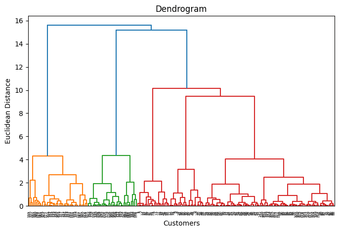
Before applying agglomerative clustering, we plot a dendrogram of our previously processed and scaled dataset: this may help us determine an optimal number of clusters (let’s just pretend for a second we forgot what our expert told us earlier).
|
plt.figure(figsize=(8, 5)) dendrogram = sch.dendrogram(sch.linkage(X_scaled, method=‘ward’)) plt.title(‘Dendrogram’) plt.xlabel(‘Customers’) plt.ylabel(‘Euclidean Distance’) plt.show() |

Once again, k=5 sounds like a good number of clusters. The reason is that if you drew a horizontal line cutting through the dendrogram at some point where vertical branches being cut are neither too distanced nor too concentrated, you would do so at the height where the dendrogram is cut five times horizontally.
Here’s how we apply the hierarchical clustering algorithm and visualize the results.
|
hc = AgglomerativeClustering(n_clusters=5, affinity=‘euclidean’, linkage=‘ward’) df[‘Cluster_HC’] = hc.fit_predict(X_scaled)
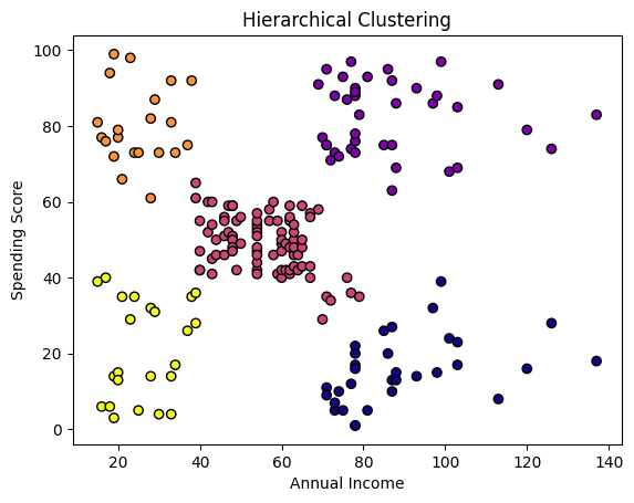
plt.scatter(X[:, 0], X[:, 1], c=df[‘Cluster_HC’], cmap=‘plasma’, edgecolors=‘k’) plt.xlabel(‘Annual Income’) plt.ylabel(‘Spending Score’) plt.title(‘Hierarchical Clustering’) plt.show() |
Besides the number of clusters sought, we also specified the affinity or similarity measure, namely Euclidean distance, as well as the linkage policy, which determines how distances between clusters are calculated: in our case, we chose ward linkage, which minimizes the variance within merged clusters for more compact grouping.

These results look very similar to those achieved with k-means, with just some subtle differences mainly in points at the boundaries between clusters.
Well done!

