

A context vector is a numerical representation of a word that captures its meaning within a specific context. Unlike traditional word embeddings that assign a single, fixed vector to each word, a context vector for the same word can change depending on the surrounding words in a sentence. Transformers are the tool of choice for generating context vectors today. In this tutorial, you’ll explore how to generate and work with context vectors using transformer models. Specifically, you will learn:
- How context vectors capture contextual information
- How to extract context vectors using a transformer model
- How to use context vectors for contextual word disambiguation
- How to visualize attention patterns in a transformer model
Let’s get started!
Generating and Visualizing Context Vectors in Transformers
Photo by Anna Tarazevich. Some rights reserved.
Overview
This post is divided into three parts; they are:
- Understanding Context Vectors
- Visualizing Context Vectors from Different Layers
- Visualizing Attention Patterns
Understanding Context Vectors
Unlike traditional word embeddings (such as Word2Vec or GloVe), which assign a fixed vector to each word regardless of context, transformer models generate dynamic representations that depend on surrounding words.
For example, in the sentences “I’m going to the bank to deposit money” and “I’m going to sit by the river bank,” the word “bank” has different meanings. A traditional word embedding would assign the same vector to “bank” in both sentences, but a transformer model generates different context vectors that capture the distinct meanings based on the surrounding words.
The power of context vectors is that they capture the meaning of words in their specific contexts, allowing you to work with the **meaning** rather than the individual words in a sentence. Context vectors are unlike word embeddings, which are retrieved from a lookup table; instead, you need a sophisticated model to generate them. Transformer models are typically used because they can produce high-quality context vectors.
Let’s see an example of how to generate context vectors from a transformer model:
|
1 2 3 4 5 6 7 8 9 10 11 12 13 14 15 16 17 18 19 20 21 22 23 24 25 26 27 28 29 30 31 32 33 34 35 36 37 38 39 40 41 42 43 44 45 46 47 48 49 50 51 52 53 |
import numpy as np import torch from transformers import BertModel, BertTokenizer
# Load pre-trained model and tokenizer tokenizer = BertTokenizer.from_pretrained(“bert-base-uncased”) model = BertModel.from_pretrained(“bert-base-uncased”) model.eval() # for safety: set to evaluation mode
def get_context_vectors(sentence, model, tokenizer): inputs = tokenizer(sentence, return_tensors=“pt”, add_special_tokens=True) input_ids = inputs[“input_ids”] attention_mask = inputs[“attention_mask”]
# Get the tokens (for reference) tokens = tokenizer.convert_ids_to_tokens(input_ids[0])
# Forward pass, get all hidden states from each layer with torch.no_grad(): outputs = model(input_ids, attention_mask=attention_mask, output_hidden_states=True) hidden_states = outputs.hidden_states
# Each element in hidden states has shape (batch_size, sequence_length, hidden_size) # Here takes the first element in the batch from the last layer last_layer_vectors = hidden_states[–1][0].numpy() # Shape: (sequence_length, hidden_size)
return tokens, last_layer_vectors
# Get context vectors from example sentences with ambiguous words sentence1 = “I’m going to the bank to deposit money.” sentence2 = “I’m going to sit by the river bank.” tokens1, vectors1 = get_context_vectors(sentence1, model, tokenizer) tokens2, vectors2 = get_context_vectors(sentence2, model, tokenizer)
# Print the tokens for reference print(“Tokens in sentence 1:”, tokens1) print(“Tokens in sentence 2:”, tokens2)
# Find the index of “bank” in both sentences bank_idx1 = tokens1.index(“bank”) bank_idx2 = tokens2.index(“bank”)
# Get the context vectors for “bank” in both sentences bank_vector1 = vectors1[bank_idx1] bank_vector2 = vectors2[bank_idx2]
# Calculate cosine similarity between the two “bank” vectors # lower similarity means meaning is different def cosine_similarity(vec1, vec2): return np.dot(vec1, vec2) / (np.linalg.norm(vec1) * np.linalg.norm(vec2))
similarity = cosine_similarity(bank_vector1, bank_vector2) print(f“Cosine similarity between ‘bank’ vectors: {similarity:.4f}”) |
This code loads a pre-trained BERT model and tokenizer. A function get_context_vectors() is defined to extract context vectors from a sentence. The function takes a sentence, passes it through the model, and collects the “hidden states” from each layer by setting output_hidden_states=True. These hidden states come from each layer of the transformer model, and all share the same shape due to the model’s consistent structure.
Typically, a transformer model includes a task-specific head (e.g., for predicting the next word in a sentence). Here, you’re not using the head; instead, you’re examining what gets passed to the head as input. If the head can make meaningful predictions, the input must already contain useful information about the sentence.
Note that the model input is a sequence of tokens, and each layer in the transformer maintains the same sequence length. Thus, once you find the position of the word “bank” in each sentence, you can extract the corresponding vector from the last hidden state and compute the cosine similarity between the two vectors.
Cosine similarity is a measure ranging from -1 to 1. A lower similarity means the meanings are more different. When you run the code, you’ll see:
|
Tokens in sentence 1: [‘[CLS]’, ‘i’, “‘”, ‘m’, ‘going’, ‘to’, ‘the’, ‘bank’, ‘to’, ‘deposit’, ‘money’, ‘.’, ‘[SEP]’] Tokens in sentence 2: [‘[CLS]’, ‘i’, “‘”, ‘m’, ‘going’, ‘to’, ‘sit’, ‘by’, ‘the’, ‘river’, ‘bank’, ‘.’, ‘[SEP]’] Cosine similarity between ‘bank’ vectors: 0.5327 |
This shows the same word “bank” is indeed quite different in the two sentences.
Visualizing Context Vectors from Different Layers
Transformer models like BERT have multiple layers, and each layer captures different aspects of the text. Like the case of computer vision using convolutional neural networks, the early layers capture low-level features (e.g., edges, corners), and the later layers capture higher-level features (e.g., shapes, objects). In the case of transformer models, the early layers capture syntactic information (e.g., whether a noun is singular or plural), and the later layers capture semantic information (what the word means in the sentence).
Since the representation changes across layers, let’s explore how to extract and analyze context vectors from different layers:
|
1 2 3 4 5 6 7 8 9 10 11 12 13 14 15 16 17 18 19 20 21 22 23 24 25 26 27 28 29 30 31 32 33 34 35 36 37 38 39 40 41 42 43 44 45 46 47 48 49 50 51 52 53 54 55 56 57 58 |
import matplotlib.pyplot as plt import numpy as np import torch from transformers import BertModel, BertTokenizer
# Load pre-trained model and tokenizer tokenizer = BertTokenizer.from_pretrained(“bert-base-uncased”) model = BertModel.from_pretrained(“bert-base-uncased”) model.eval() # for safety: set to evaluation mode
def get_all_layer_vectors(sentence, model, tokenizer): inputs = tokenizer(sentence, return_tensors=“pt”, add_special_tokens=True) input_ids = inputs[“input_ids”] attention_mask = inputs[“attention_mask”]
# Get the tokens (for reference) tokens = tokenizer.convert_ids_to_tokens(input_ids[0])
# Forward pass, get all hidden states from each layer with torch.no_grad(): outputs = model(input_ids, attention_mask=attention_mask, output_hidden_states=True) hidden_states = outputs.hidden_states
# Convert from torch tensor to numpy arrays, take only the first element in the batch all_layers_vectors = [layer[0].numpy() for layer in hidden_states]
return tokens, all_layers_vectors
# Get vectors from all layers for a sentence sentence = “The quick brown fox jumps over the lazy dog.” tokens, all_layers = get_all_layer_vectors(sentence, model, tokenizer) print(f“Number of layers (including embedding layer): {len(all_layers)}”)
# Let’s analyze how the representation of a word changes across layers word = “fox” word_idx = tokens.index(word)
# Extract the vector for this word from each layer word_vectors_across_layers = [layer[word_idx] for layer in all_layers]
# Calculate the cosine similarity between consecutive layers def cosine_similarity(vec1, vec2): return np.dot(vec1, vec2) / (np.linalg.norm(vec1) * np.linalg.norm(vec2))
similarities = [] for i in range(len(word_vectors_across_layers) – 1): sim = cosine_similarity(word_vectors_across_layers[i], word_vectors_across_layers[i+1]) similarities.append(sim)
# Plot the similarities plt.figure(figsize=(10, 6)) plt.plot(similarities, marker=‘o’) plt.title(f“Cosine Similarity Between Consecutive Layers for ‘{word}'”) plt.xlabel(‘Layer Transition’) plt.ylabel(‘Cosine Similarity’) plt.xticks(range(len(similarities)), [f“{i}->{i+1}” for i in range(len(similarities))]) plt.grid(True) plt.show() |
This code uses the same model as the previous example, with a similar flow. The function get_all_layer_vectors() returns hidden states from all layers in NumPy array format, rather than just the last layer.
Each hidden state is a tensor of shape (batch size, sequence length, hidden dimension). The token sequence is transformed by each layer, but the sequence length remains the same. So, once you’ve located the target word in the sentence, you can extract its corresponding vector from each layer.
The code calculates the cosine similarity of a selected word’s vector across consecutive layers. When you run it, you’ll see:
|
Number of layers (including embedding layer): 13 |
and the resulting plot of cosine similarity between layers:
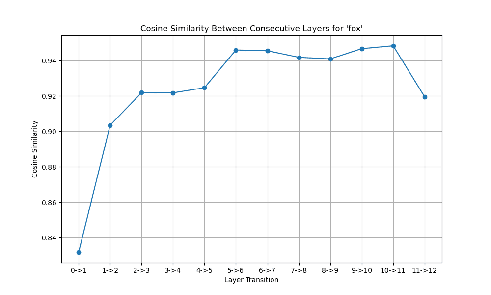
Plot showing how the context vector changes between layers in a model
You’ll notice that the word’s representation changes significantly in early layers but stabilizes later. This supports the idea that earlier layers handle syntactic features, while later ones refine semantic meaning.
Contextual Word Disambiguation
One of the most powerful applications of context vectors is word sense disambiguation: determining which meaning of a word is being used in a given context. This helps identify how many distinct senses a word can have. Let’s implement a simple word sense disambiguation system using context vectors:
|
1 2 3 4 5 6 7 8 9 10 11 12 13 14 15 16 17 18 19 20 21 22 23 24 25 26 27 28 29 30 31 32 33 34 35 36 37 38 39 40 41 42 43 44 45 46 47 48 49 50 51 52 53 54 55 56 57 58 59 60 61 62 63 64 65 66 67 68 69 70 71 72 73 74 75 76 77 78 79 80 81 82 83 84 85 86 87 88 89 |
import numpy as np import torch from transformers import BertModel, BertTokenizer
# Load pre-trained model and tokenizer tokenizer = BertTokenizer.from_pretrained(“bert-base-uncased”) model = BertModel.from_pretrained(“bert-base-uncased”) model.eval() # for safety: set to evaluation mode
def get_context_vectors(sentence, model, tokenizer): inputs = tokenizer(sentence, return_tensors=“pt”, add_special_tokens=True) input_ids = inputs[“input_ids”] attention_mask = inputs[“attention_mask”]
# Get the tokens (for reference) tokens = tokenizer.convert_ids_to_tokens(input_ids[0])
# Forward pass, get all hidden states from each layer with torch.no_grad(): outputs = model(input_ids, attention_mask=attention_mask, output_hidden_states=True) hidden_states = outputs.hidden_states
# Each element in hidden states has shape (batch_size, sequence_length, hidden_size) # Here takes the first element in the batch from the last layer last_layer_vectors = hidden_states[–1][0].numpy() # Shape: (sequence_length, hidden_size)
return tokens, last_layer_vectors
def cosine_similarity(vec1, vec2): return np.dot(vec1, vec2) / (np.linalg.norm(vec1) * np.linalg.norm(vec2))
def disambiguate_word(word, sentences, model, tokenizer): “”“for word sense disambiguation”“”
# Get context vector of a word for each sentence word_vectors = [] for sentence in sentences: tokens, vectors = get_context_vectors(sentence, model, tokenizer) for token_index, token in enumerate(tokens): if token == word: word_vectors.append({ ‘sentence’: sentence, ‘vector’: vectors[token_index] })
# Calculate pairwise similarities between all vectors n = len(word_vectors) similarity = np.zeros((n, n)) for i in range(n): for j in range(i, n): value = cosine_similarity(word_vectors[i][‘vector’], word_vectors[j][‘vector’]) similarity[i, j] = similarity[j, i] = value
# Run simple clustering to group vectors of high similarity threshold = 0.60 # Similarity > threshold will be the same cluster clusters = []
for i in range(n): # Check if this vector belongs to any existing cluster assigned = False for cluster in clusters: # Calculate average similarity with all vectors in the cluster avg_sim = np.mean([similarity[i, j] for j in cluster]) if avg_sim > threshold: cluster.append(i) assigned = True break # If not assigned to any cluster, create a new one if not assigned: clusters.append([i])
# Print the results print(f“Found {len(clusters)} different senses for ‘{word}’:\n”) for i, cluster in enumerate(clusters): print(f“Sense {i+1}:”) for idx in cluster: print(f” – {word_vectors[idx][‘sentence’]}”) print()
# Example: Disambiguate the word “bank” sentences = [ “I’m going to the bank to deposit money.”, “The bank approved my loan application.”, “I’m going to sit by the river bank.”, “The bank of the river was muddy after the rain.”, “The central bank raised interest rates yesterday.”, “They had to bank the fire to keep it burning through the night.” ] disambiguate_word(“bank”, sentences, model, tokenizer) |
In this example, you define a function disambiguate_word() that takes a target word and a list of sentences containing that word. The function converts each sentence into context vectors using get_context_vectors() and extracts the vector corresponding to the target word.
With all the context vectors of the same word gathered, you compute cosine similarities between every pair and perform clustering to group similar ones. The clustering algorithm used here is basic and threshold-based. You can improve it by using more sophisticated methods like K-means or hierarchical clustering—available in the scikit-learn library—or incorporating additional features.
The result of the clustering is printed. If you run the code, you will see:
|
Found 3 different senses for ‘bank’:
Sense 1: – I’m going to the bank to deposit money. – The bank approved my loan application. – The central bank raised interest rates yesterday.
Sense 2: – I’m going to sit by the river bank. – The bank of the river was muddy after the rain.
Sense 3: – They had to bank the fire to keep it burning through the night. |
While the output doesn’t explicitly label the meanings, you can observe that different senses of the word “bank” are identified: as a financial institution, the side of a river, or a verb meaning to support or save from destruction. This demonstrates how context vectors can be used for word sense disambiguation.
This shows that the word “bank” indeed has different representations in these sentences.
Visualizing Attention Patterns
Another way to understand how transformer models process text is by visualizing their attention patterns. The attention mechanism allows transformers to weigh the importance of different words when generating context vectors. In other words, attention weights show how much each word “attends to” other words in the sentence.
Let’s implement a tool to visualize attention:
|
1 2 3 4 5 6 7 8 9 10 11 12 13 14 15 16 17 18 19 20 21 22 23 24 25 26 27 28 29 30 31 32 33 34 35 36 37 38 39 40 41 42 43 44 45 46 47 48 49 50 51 52 53 54 55 56 57 58 59 60 61 62 63 64 65 66 67 68 69 70 71 72 73 74 75 76 77 78 79 |
import matplotlib.pyplot as plt import numpy as np import seaborn as sns import torch from transformers import BertTokenizer, BertModel
# Load pre-trained model and tokenizer tokenizer = BertTokenizer.from_pretrained(“bert-base-uncased”) model = BertModel.from_pretrained(“bert-base-uncased”) model.eval() # for safety: set to evaluation mode
def get_attention_weights(sentence, model, tokenizer): inputs = tokenizer(sentence, return_tensors=“pt”, add_special_tokens=True) input_ids = inputs[“input_ids”] attention_mask = inputs[“attention_mask”]
# Get the tokens (for reference) tokens = tokenizer.convert_ids_to_tokens(input_ids[0])
# Forward pass, get attention weights with torch.no_grad(): outputs = model(input_ids, attention_mask=attention_mask, output_attentions=True)
# One weight for each attention layer in the model # Each element in has shape (batch_size, num_heads, sequence_length, sequence_length) attentions = outputs.attentions
return tokens, attentions
def visualize_attention(tokens, attention_weights, layer, head): “”“visualize attention for a specific layer and head”“”
# Get attention weights for the specified layer and head # Shape: (sequence_length, sequence_length) attn = attention_weights[layer][0, head].numpy()
# Create a figure and axis fig, ax = plt.subplots(figsize=(10, 8))
# Create a heatmap sns.heatmap(attn, xticklabels=tokens, yticklabels=tokens, cmap=“viridis”, ax=ax) ax.set_title(f“Attention Weights – Layer {layer+1}, Head {head+1}”) ax.set_xlabel(“Token (Key)”) ax.set_ylabel(“Token (Query)”) plt.xticks(rotation=90) # Rotate x-axis labels for better readability plt.tight_layout() plt.show()
def visualize_layer_attention(tokens, attention_weights, layer): “”“visualize the average attention across all heads for a layer”“”
# Get average attention weights across all heads for the specified layer # Shape: (sequence_length, sequence_length) attn = attention_weights[layer][0].mean(dim=0).numpy()
# Create a figure and axis fig, ax = plt.subplots(figsize=(10, 8))
# Create a heatmap sns.heatmap(attn, xticklabels=tokens, yticklabels=tokens, cmap=“viridis”, ax=ax) ax.set_title(f“Average Attention Weights – Layer {layer+1}”) ax.set_xlabel(“Token (Key)”) ax.set_ylabel(“Token (Query)”) plt.xticks(rotation=90) # Rotate x-axis labels for better readability plt.tight_layout() plt.show()
# Get attention weight from an example sentence sentence = “The president of the United States visited the capital city.” tokens, attention_weights = get_attention_weights(sentence, model, tokenizer)
# Visualize attention for a specific layer and head # BERT base has 12 layers (0-11) and 12 heads per layer (0-11) layer_to_visualize = 5 # 6th layer (0-indexed) head_to_visualize = 7 # 8th attention head (0-indexed) visualize_attention(tokens, attention_weights, layer_to_visualize, head_to_visualize)
# Visualize average attention for a layer visualize_layer_attention(tokens, attention_weights, layer_to_visualize) |
When you run this code, two heatmaps will be generated:
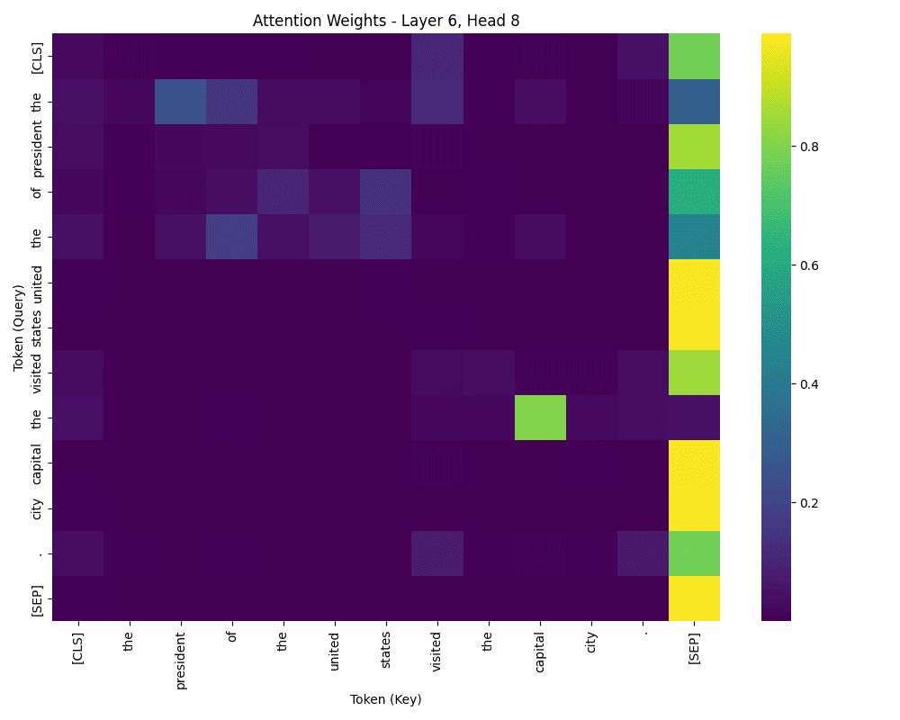
Attention weights from one head

Average attention weights from one layer
The first heatmap shows the attention weights for a specific layer and head. The x-axis represents the “key” tokens, and the y-axis represents the “query” tokens. Brighter colors indicate stronger attention.
The second heatmap shows the average attention weights across all heads in a layer.
The attention data is obtained by setting output_attentions=True when invoking the model. Each head produces a square matrix of attention weights, which is a by-product of each transformer layer and not pass on from one layer to another. Each element in the matrix indicates the attention from one token to another. The lower the weight, the less attention the query token gives to the key token.
Attention weights are not symmetric, as query and key tokens serve different roles. The query token is the one being processed, and the key token is the one being referenced. In the first heatmap, for example, the word “of” may attend strongly to “the,” “united,” and “states”—but not necessarily the other way around. Interestingly, “the” might also attend strongly to “of,” indicating bidirectional attention in certain cases.
While it’s not always obvious why the model attends the way it does, especially since different heads may specialize in different roles, a close inspection can reveal patterns. Some heads may focus on syntax, others on semantics or named entities. If you visualize a different layer or head, the heatmap may look entirely different.
In the second heatmap, attention is averaged across all heads, providing a general view of how words relate to one another in the sentence. The stronger the attention between two words, the stronger their modeled relationship.
These visualizations offer insights into how the model interprets and processes text.
Further Reading
Below are some further readings that you might find useful:
Summary
In this post, you learned how to generate and visualize context vectors using transformer models. Specifically, you explored:
- How context vectors capture contextual information
- How to extract context vectors using a transformer model
- How to use context vectors for contextual word disambiguation
- How to visualize attention patterns in a transformer model