

Transformer is a deep learning architecture that is very popular in natural language processing (NLP) tasks. It is a type of neural network that is designed to process sequential data, such as text. In this article, we will explore the concept of attention and the transformer architecture. Specifically, you will learn:
- What problems do the transformer models address
- What is the relationship of attention to transformer models
- What are the different variations in the transformer models
Let’s get started!
A Gentle Introduction to Attention and Transformer Models
Photo by Andre Benz. Some rights reserved.
Overview
This post is divided into three parts; they are:
- Origination of the Transformer Model
- The Transformer Architecture
- Variations of the Transformer Architecture
Origination of the Transformer Model
Transformer architecture originated from the 2017 paper “Attention is All You Need” by Vaswani et al. It is different from traditional neural networks in that it uses self-attention mechanisms to process the input data. Self-attention mechanisms allow the model to focus on different parts of the input data, depending on the task’s needs.
Transformer architecture addresses the limitations of recurrent neural networks (RNNs). RNNs are expected to process a sequence of input, such as a sequence of vectors. The same network architecture is used repeatedly to process each element of the sequence. Inside the network, some memory mechanism is used. The memory is updated at each step, representing the sequence seen so far.
RNNs are useful in NLP tasks, such as seq2seq architectures, to translate natural language. However, since RNNs process one element at a time, it is difficult for the network to remember the information delivered by the first element while the last element of the sequence is being processed, especially when the sequence is arbitrarily long.
The solution in the transformer architecture is to allow the entire sequence to be processed at once using the self-attention mechanism. Each element of the sequence can “see” all elements in the sequence, and the model can extract the information within the context. Therefore, the transformer architecture can perform better. Moreover, the nature of the attention mechanism allows the computation to be more parallelizable since, unlike RNNs, the output corresponding to one element of the sequence does not depend on the output corresponding to other elements of the sequence.
The Transformer Architecture
The original transformer architecture is composed of an encoder and a decoder. Its layout is shown in the figure below.
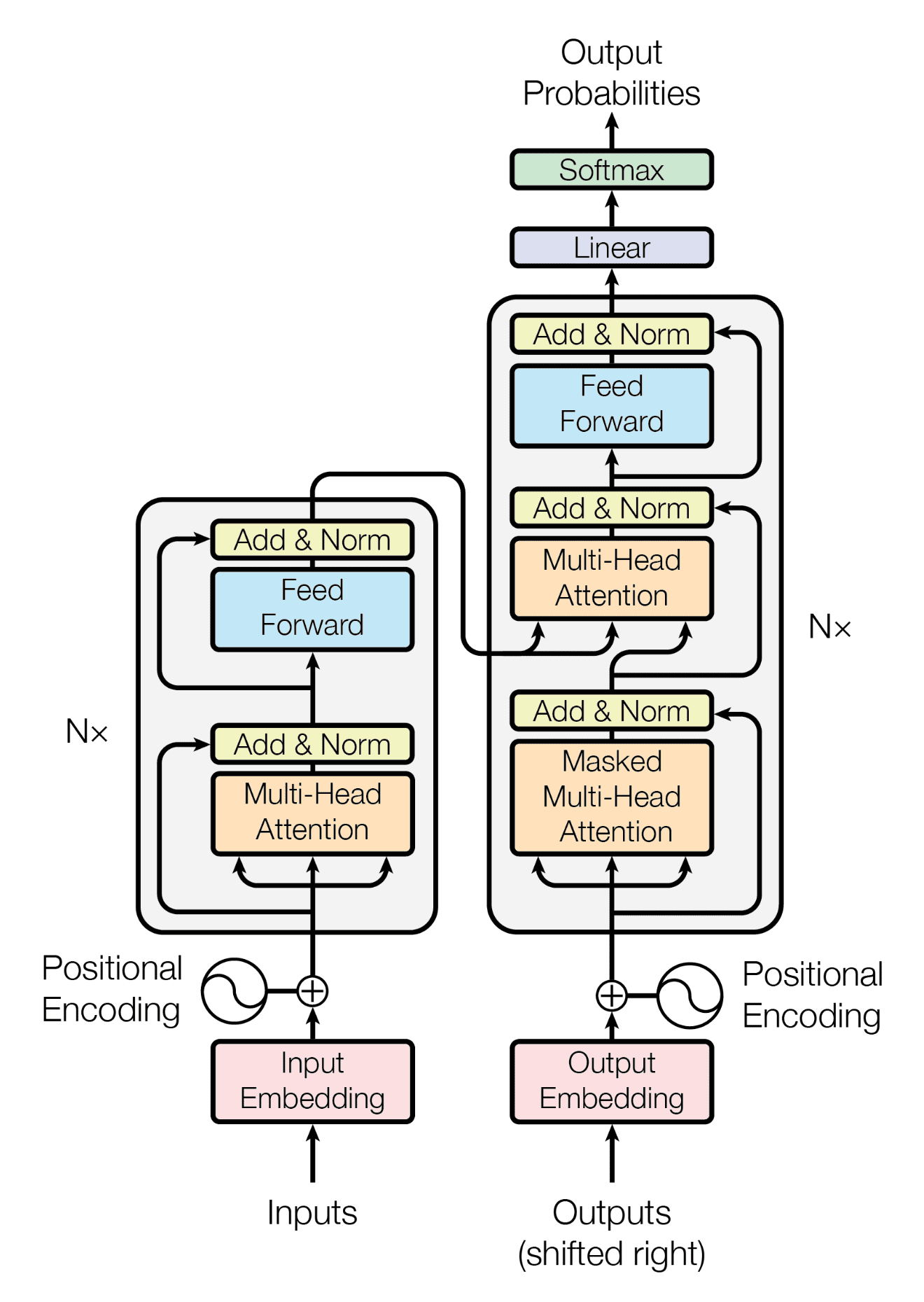
Recall that the transformer model was developed for translation tasks, replacing the seq2seq architecture that was commonly used with RNNs. Therefore, it borrowed the encoder-decoder architecture.
The encoder is used to encode the input data, i.e., the sentence in the source language. The encoder outputs a context representation of the input sentence that supposedly captures the meaning of the sentence.
The decoder is used to produce the output, i.e., to generate the sentence in the target language, capturing the same meaning as the sentence in the source language. Therefore, the decoder takes the context representation from the encoder as one of the inputs. The decoder produces one word (technically called a token) of the target sentence at a time. It needs to know what was generated so far to determine what to generate next. Hence the partial sequence generated so far is fed back to the decoder as another input.
Usually, the encoder and decoder in a transformer model are composed of a stack of identical layers. Each layer, in both the encoder and the decoder, is an attention sublayer followed by a feed-forward sublayer.
The attention sublayer transforms the input sequence, one element at a time, by “attending” each element to every other element in the sequence. It behaves like a lookup table to find the most appropriate output. It is a linear transformation in nature, and the output is a sequence of the same length as the input. The feed-forward sublayer, however, is a non-linear transformation. It is a multi-layer perceptron with an activation function to apply to each element of the sequence.
In essence, the attention layer allows each element of the sequence to learn from all other elements in the sequence, then the feed-forward layer further transformed each element.
The modern attention mechanism used in the transformer architecture is called Scaled Dot-Product Attention. It takes three input sequences: a query, a key, and a value. The query and key compute the attention weights, which are then used to compute the weighted sum of the value as the output.
Usually, the attention used in the encoder layers is self-attention, meaning that the same input sequence is used to derive the query, key, and value sequences. In decoder layers, however, both self-attention and cross-attention are used. The cross-attention in the decoder uses the partially generated sequence as the query and the context representation from the encoder as the key and value.
Variations of the Transformer Architecture
Let’s look at how an encoder layer in the transformer architecture is implemented.
|
1 2 3 4 5 6 7 8 9 10 11 12 13 14 15 16 17 18 19 20 21 22 23 24 25 26 27 28 29 30 31 32 33 34 35 36 37 38 39 40 |
import torch import torch.nn as nn
class TransformerEncoderLayer(nn.Module): def __init__(self, d_model, d_ff, num_heads): super().__init__() self.attention = nn.MultiheadAttention(d_model, num_heads, batch_first=True) self.ff_proj = nn.Linear(d_model, d_ff) self.output_proj = nn.Linear(d_ff, d_model) self.norm1 = nn.LayerNorm(d_model) self.norm2 = nn.LayerNorm(d_model) self.act = nn.ReLU()
def forward(self, x): “”“Process the input sequence x
Args: x (torch.Tensor): The input sequence of shape (batch_size, seq_len, d_model).
Returns: torch.Tensor: The processed sequence of shape (batch_size, seq_len, d_model). ““” # Self-attention sublayer residual = x x = self.attention(x, x, x) x = self.norm1(x[0] + residual)
# Feed-forward sublayer residual = x x = self.act(self.ff_proj(x)) x = self.act(self.output_proj(x)) x = self.norm2(x + residual)
return x
seq = torch.randn(3, 7, 16) layer = TransformerEncoderLayer(16, 32, 4) out_seq = layer(seq) print({name: weight.shape for name, weight in layer.state_dict().items()}) print(out_seq.shape) |
This is a simplified implementation in which a lot of minor details and error handling are removed. In essence, the input sequence is a tensor of shape (batch_size, seq_len, d_model), where d_model is the dimension of the model or the size of each vector element in the sequence. The output sequence is of the same shape so you can process it again with another encoder layer. Therefore, you can easily stack up multiple layers to form the encoder.
The MultiheadAttention layer produces a Python tuple. The first element is the attention output, and the second is the attention weights, which are not used in this implementation. Then, the output is added back to the original input, and a layer normalization is applied. Adding the output back to the input is called a residual connection. It is a common practice in deep learning to help the model learn better.
After the attention sublayer, the output sequence is passed to a feed-forward sublayer. The feed-forward sublayer is a multi-layer perceptron with a ReLU activation function to process each element separately. The output is again the same shape as the input sequence, although a larger dimension is usually used in the middle.
The output from the feed-forward sublayer will have another residual connection and normalization. Then this is the output of the encoder layer.
The code above illustrates the post-norm architecture. This is the architecture proposed by the original transformer paper, but later, it was found that the pre-norm architecture is easier to train. The pre-norm version is like the following:
|
1 2 3 4 5 6 7 8 9 10 11 12 13 14 15 16 17 18 19 20 21 22 23 24 25 26 27 28 29 30 31 32 33 34 35 36 37 38 39 40 41 42 |
import torch import torch.nn as nn
class TransformerEncoderLayer(nn.Module): def __init__(self, d_model, d_ff, num_heads): super().__init__() self.attention = nn.MultiheadAttention(d_model, num_heads, batch_first=True) self.ff_proj = nn.Linear(d_model, d_ff) self.output_proj = nn.Linear(d_ff, d_model) self.norm1 = nn.LayerNorm(d_model) self.norm2 = nn.LayerNorm(d_model) self.act = nn.ReLU()
def forward(self, x): “”“Process the input sequence x
Args: x (torch.Tensor): The input sequence of shape (batch_size, seq_len, d_model).
Returns: torch.Tensor: The processed sequence of shape (batch_size, seq_len, d_model). ““” # Self-attention sublayer residual = x x = self.norm1(x) x = self.attention(x, x, x) x = x[0] + residual
# Feed-forward sublayer residual = x x = self.norm2(x) x = self.act(self.ff_proj(x)) x = self.act(self.output_proj(x)) x = x + residual
return x
seq = torch.randn(3, 7, 16) layer = TransformerEncoderLayer(16, 32, 4) out_seq = layer(seq) print({name: weight.shape for name, weight in layer.state_dict().items()}) print(out_seq.shape) |
You always have the residual connection after the attention or feed-forward sublayer. But in the pre-norm architecture, the layer normalization is applied at the beginning of the sublayer rather than at the end.
In the two example codes above, the output is always the following:
|
{‘attention.in_proj_bias’: torch.Size([48]), ‘attention.in_proj_weight’: torch.Size([48, 16]), ‘attention.out_proj.bias’: torch.Size([16]), ‘attention.out_proj.weight’: torch.Size([16, 16]), ‘ff_proj.bias’: torch.Size([32]), ‘ff_proj.weight’: torch.Size([32, 16]), ‘norm1.bias’: torch.Size([16]), ‘norm1.weight’: torch.Size([16]), ‘norm2.bias’: torch.Size([16]), ‘norm2.weight’: torch.Size([16]), ‘output_proj.bias’: torch.Size([16]), ‘output_proj.weight’: torch.Size([16, 32])} torch.Size([3, 7, 16]) |
It is easy to identify the weights for the two linear layers and the two normalization layers. The weights for the attention layer are in two parts: The input projection and the output projection. The input projection has a shape of $48\times 16$, and the output projection has a shape of $16\times 16$. The 48 comes from the fact that the input to the attention layer is the concatenation of the query, key, and value sequences, each of which has a shape of batch_size, seq_len, d_model with d_model=16. Hence $16\times 3=48$.
You cannot see the effect of num_heads=4 in the weights because when you set d_model, the dimension of each head is d_model/num_heads. Thus, each attention head, in this case, only handles the dimension of 4. Each head processes one slice of the projected input and then concatenates along the embedding dimension to form the final output.
The feed-forward layers in these examples use ReLU as the activation function. You can use other activation functions, such as GELU or SwiGLU. In fact, modern transformer models are less likely to use ReLU.
Layer normalization is applied in these examples. Some models will use the RMS norm instead.
The implementation for decoder layers is similar. Except you need to add a cross-attention layer and invoke it differently:
|
x = self.attention(x, y, y) |
where y is the sequence from the encoder output, and it can be of a different length. In full, the code is like the following:
|
1 2 3 4 5 6 7 8 9 10 11 12 13 14 15 16 17 18 19 20 21 22 23 24 25 26 27 28 29 30 31 32 33 34 35 36 37 38 39 40 41 42 43 44 45 46 47 48 49 50 51 52 |
import torch import torch.nn as nn
class TransformerDecoderLayer(nn.Module): def __init__(self, d_model, d_ff, num_heads): super().__init__() self.attention = nn.MultiheadAttention(d_model, num_heads, batch_first=True) self.xattention = nn.MultiheadAttention(d_model, num_heads, batch_first=True) self.ff_proj = nn.Linear(d_model, d_ff) self.output_proj = nn.Linear(d_ff, d_model) self.norm1 = nn.LayerNorm(d_model) self.norm2 = nn.LayerNorm(d_model) self.norm3 = nn.LayerNorm(d_model) self.act = nn.ReLU()
def forward(self, x, y): “”“Process the input sequence x with decoder input y
Args: x (torch.Tensor): The input sequence of shape (batch_size, seq_len, d_model). y (torch.Tensor): The output sequence from encoder of shape (batch_size, seq_len, d_model).
Returns: torch.Tensor: The processed sequence of shape (batch_size, seq_len, d_model). ““” # Self-attention sublayer residual = x x = self.norm1(x) x = self.attention(x, x, x) x = x[0] + residual
# Cross-attention sublayer residual = x x = self.norm2(x) x = self.xattention(x, y, y) x = x[0] + residual
# Feed-forward sublayer residual = x x = self.norm3(x) x = self.act(self.ff_proj(x)) x = self.act(self.output_proj(x)) x = x + residual
return x
dec_seq = torch.randn(3, 7, 16) enc_seq = torch.randn(3, 11, 16) layer = TransformerDecoderLayer(16, 32, 4) out_seq = layer(dec_seq, enc_seq) print({name: weight.shape for name, weight in layer.state_dict().items()}) print(out_seq.shape) |
Further Reading
Below are some papers that you may find useful.
Summary
In this article, you learned about the transformer architecture and the attention mechanism. You have also seen how to implement the encoder and decoder layers in PyTorch. In particular, you learned:
- The transformer architecture is a type of neural network that is designed to process sequential data, such as text.
- A signature of transformer models is the use of attention mechanisms to process the input sequence.
- The transformer architecture is composed of an encoder and a decoder. Each is a stack of identical layers.
- With a similar architecture, the transformer model can have variations in pre-norm or post-norm, different normalization methods, and different activation functions.
Learn Transformers and Attention!
Teach your deep learning model to read a sentence
…using transformer models with attention
Discover how in my new Ebook:
Building Transformer Models with Attention
It provides self-study tutorials with working code to guide you into building a fully-working transformer models that can
translate sentences from one language to another…